Implementation¶

Separable prior¶

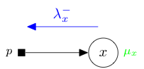
A prior has one output variable here denoted \(x\). In a message passing context, for instance in expectation propagation or state evolution, it receives a natural parameter message \(\lambda_x^-\) coming from \(x\) and returns a moment \(\mu_x\).

We detail below how to derive mathematically, and implement concretely in Tree-AMP, a prior for:

Sampling
Expectation propagation
Second moment
State evolution

All priors share the same implementation, however MAP priors and Committee priors require some special handling. Please consult the revelant section if need be.

Tip

When you create a new prior, you do not have to implement all the methods simultaneously. If you want to postpone the mathematical derivation or implementation just raise an NotImplementedError in the corresponding method.

Sampling¶

A prior is implemented in Tree-AMP as a subclass of the base Prior class. The constructor prior.__init__() must contain as parameters:

the size which corresponds to the shape of the variable \(x\),
the isotropic flag for isotropic/diagonal beliefs in EP,
additional parameters needed to specify the prior.

See the GaussBernoulliPrior class, both its documentation and source code, for an example.

>>> from tramp.priors import GaussBernoulliPrior
>>> prior = GaussBernoulliPrior(size=100)
>>> print(prior)
GaussBernoulliPrior(size=100,rho=0.5,mean=0,var=1,isotropic=True)

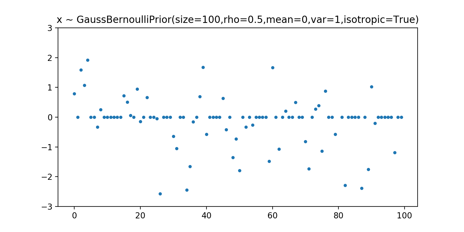
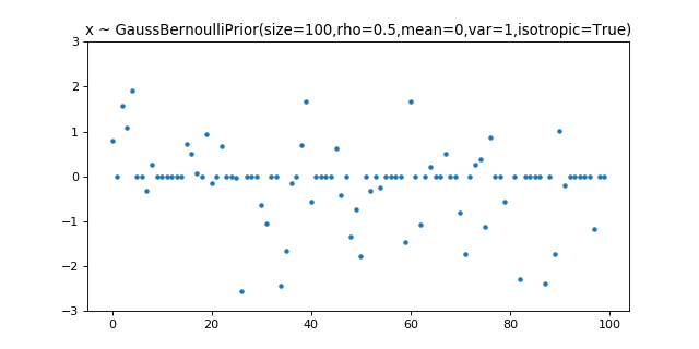
The prior.sample() method takes no arguments and must return a sample \(x\) of shape size from the prior.

>>> import matplotlib.pyplot as plt
>>> # sample x
>>> x = prior.sample()
>>> assert x.shape == (100,)
>>> # plot x
>>> fig, axs = plt.subplots(1, 1, figsize=(8, 4))
>>> axs.plot(x, '.')
>>> axs.set(title=f"x ~ {prior}", ylim=(-3, 3));

(png, hires.png, pdf)

Expectation propagation¶

Note

We are only considering separable priors \(p(x) = \prod_{i=1}^{N_x} p(x^{[i]})\) in this section. For an example of a non separable prior see the MAP L21 norm prior.

Scalar quantities¶

The scalar EP log-partition, mean and variance are given by:

\[A_p[a_x^-,b_x^-] = \ln \int dx \, p(x) \, e^{-\frac{1}{2} a_x^- x^2 + b_x^- x} , \quad r_x[a_x^-,b_x^-] = \partial_{b_x^-} A_p[a_x^-,b_x^-] , \quad v_x[a_x^-,b_x^-] = \partial^2_{b_x^-} A_p[a_x^-,b_x^-] ,\]

and are implemented in Tree-AMP as the methods:

prior.scalar_log_partition() for \(A_p[a_x^-,b_x^-]\),
prior.scalar_forward_mean() for \(r_x[a_x^-,b_x^-]\),
prior.scalar_forward_variance() for \(v_x[a_x^-,b_x^-]\).

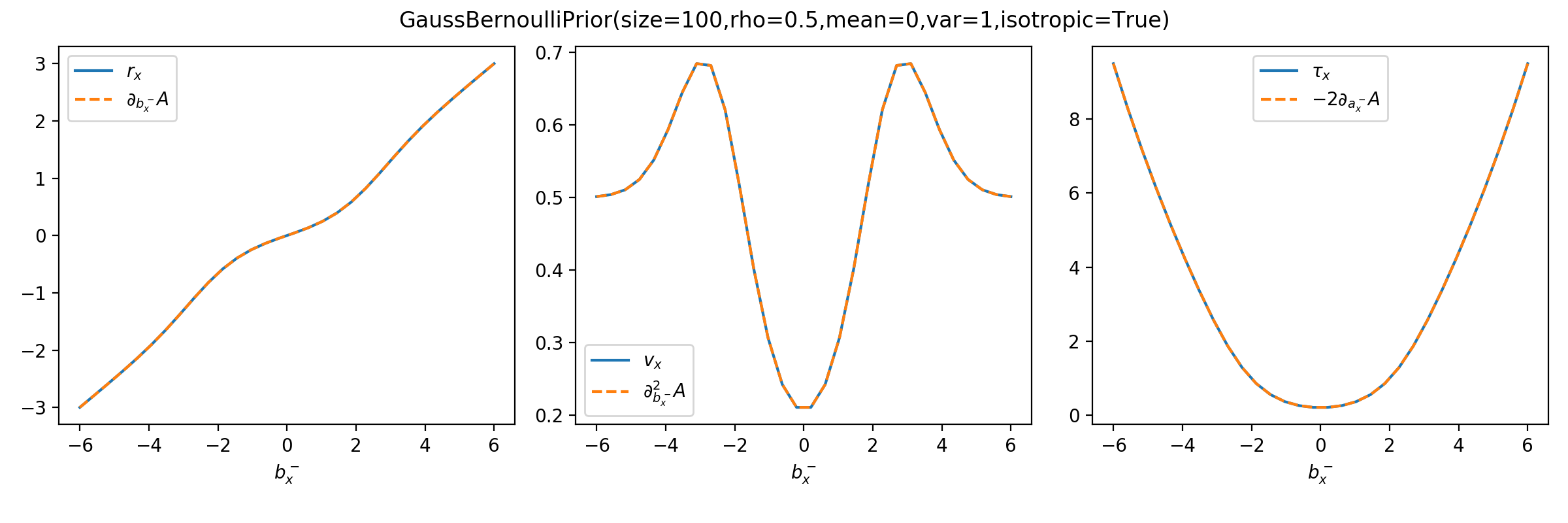
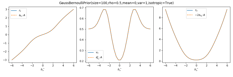
As a sanity check, you can use tramp.checks.plot_prior_grad_EP() to check the gradients \(r_x = \partial_{b_x^-} A_p\), \(v_x = \partial^2_{b_x^-} A_p\) and \(\tau_x = r_x^2 + v_x = -2 \partial_{a_x^-} A_p\).

>>> from tramp.checks import plot_prior_grad_EP_scalar
>>> plot_prior_grad_EP_scalar(prior)

(png, hires.png, pdf)

Diagonal beliefs¶

During expectation propagation, when using diagonal beliefs prior.isotropic=False, the prior receives the natural parameter message \(\lambda_x^-=b_x^- a_x^-\) and returns the moment \(\mu_x = r_x v_x\) where \(b_x^-\), \(a_x^-\), \(r_x\) and \(v_x\) are all arrays of the same shape size as the variable \(x\). For a separable prior, the corresponding log-partition, mean and variance vectorize their scalar counterparts:

\[A_p[a_x^-,b_x^-] = \frac{1}{N_x} \sum_{i=1}^{N_x} A_p[a_x^{-[i]},b_x^{-[i]}], \quad r_x^{[i]}[a_x^-,b_x^-] = r_x[a_x^{-[i]},b_x^{-[i]}], \quad v_x^{[i]}[a_x^-,b_x^-] = v_x[a_x^{-[i]},b_x^{-[i]}],\]

and are implemented in Tree-AMP by the methods:

prior.compute_log_partition() for \(A_p[a_x^-,b_x^-]\),
prior.compute_forward_posterior() for \(r_x[a_x^-,b_x^-]\) and \(v_x[a_x^-,b_x^-]\).

Actually only the vectorized versions are used in EP. However it is useful to also provide the scalar versions which are used in SE and in the gradient checking.

Isotropic beliefs¶

When using isotropic beliefs prior.isotropic=True, the only difference is that the precision \(a_x^-\) and variance \(v_x\) are scalars instead of vectors. For the implementation, this means that prior.compute_forward_posterior() must return the scalar variance \(v_x = \frac{1}{N_x} \sum_{i=1}^{N_x} v_x^{[i]}\) averaged over components when prior.isotropic=True.

Tests¶

If you implement a new prior for EP, please add it to the test suite tramp.tests.test_priors to make sure that it passes the vectorization test_separable_prior_vectorization() and the gradient checking test_prior_grad_EP_scalar().

Second moment¶

Factor graph¶

When the teacher generative model is a factor graph, the prior log-partition and second moment are given by:

\[A_p[\hat{\tau}_x^-] = \ln \int dx \, p(x) \, e^{-\frac{1}{2} \hat{\tau}_x^- x^2 } , \quad \tau_x[\hat{\tau}_x^-] = - 2 \partial_{\hat{\tau}_x^-} A_p[\hat{\tau}_x^-] ,\]

and are implemented in Tree-AMP by the methods:

prior.prior_log_partition_FG() for \(A_p[\hat{\tau}_x^-]\),
prior.forward_second_moment_FG() for \(\tau_x[\hat{\tau}_x^-]\).

The prior log-partition is easily obtained from the scalar EP one \(A_p[\hat{\tau}_x^-] = A_p[a_x^- = \hat{\tau}_x^-, b_x^- =0]\) and the prior.prior_log_partition_FG() method is already implemented in the base Prior class. When you create a new prior, you therefore only need to implement the prior.forward_second_moment_FG() method.

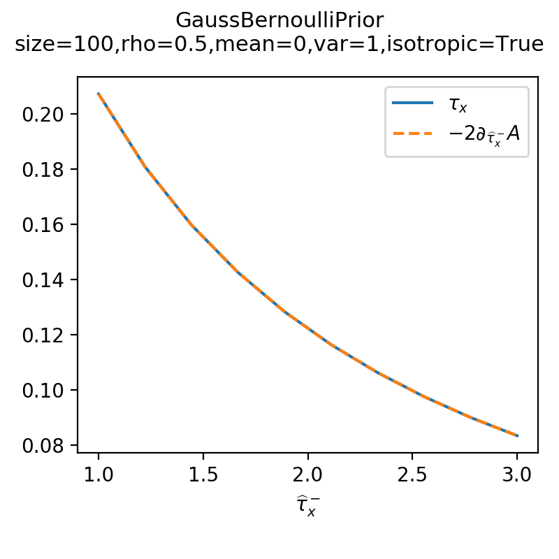
As a sanity check, you can use tramp.checks.plot_prior_grad_FG() to check the gradient \(\tau_x = -2 \partial_{\hat{\tau}_x^-} A_p\).

>>> from tramp.checks import plot_prior_grad_FG
>>> plot_prior_grad_FG(prior)

(png, hires.png, pdf)

Bayesian network¶

When the teacher generative model is a Bayesian network, we have \(\hat{\tau}_x^- =0\). Then the prior second-moment is simply given by:

\[\tau_x = \mathbb{E}_{p(x)} x^2\]

and is implemented in Tree-AMP by the method prior.second_moment().

Tests¶

If you implement a new prior, please add it to the test suite tramp.tests.test_priors to make sure that it passes the gradient checking test_prior_grad_FG().

State evolution¶

Replica symmetric¶

In the replica symmetric but mismatched case, the teacher generative model (a factor graph) will differ from the student one by some of its factors. In particular the teacher prior \(p^{(0)}(x)\) can be different from the student prior \(p(x)\). The ensemble average log-partition (free entropy), overlap \(m_x\), self-overlap \(q_x\) and variance \(v_x\) are given by:

\[\begin{split}&A_p[\hat{m}_x^-,\hat{q}_x^-,\hat{\tau}_x^-] = \mathbb{E}_{ p^{(0)}(x, b_x^-) } \, A_p[a_x^-,b_x^-] ,\\ &m_x[\hat{m}_x^-,\hat{q}_x^-,\hat{\tau}_x^-] = \mathbb{E}_{ p^{(0)}(x, b_x^-) } \, x r_x[a_x^-,b_x^-] ,\\ &q_x[\hat{m}_x^-,\hat{q}_x^-,\hat{\tau}_x^-] = \mathbb{E}_{ p^{(0)}(x, b_x^-) } \, r_x^2[a_x^-,b_x^-] ,\\ &v_x[\hat{m}_x^-,\hat{q}_x^-,\hat{\tau}_x^-] = \mathbb{E}_{ p^{(0)}(x, b_x^-) } \, v_x[a_x^-,b_x^-] ,\end{split}\]

with \(a_x^- = \hat{q}_x^- + \hat{\tau}_x^-\) and

\[p^{(0)}(x, b_x^-) = p^{(0)}(x ; \hat{\tau}_x^{-(0)}) \mathcal{N}(b_x^- | \hat{m}_x^- x, \hat{q}_x^-) , \quad p^{(0)}(x ; \hat{\tau}_x^{-(0)} ) = p^{(0)}(x) e^{ -\frac{1}{2} \hat{\tau}_x^{-(0)} x^2 - A_{p^{(0)}}[\hat{\tau}_x^{-(0)}] } ,\]

and are already implemented in the base Prior class as the methods:

prior.compute_potential_RS() for \(A_p[\hat{m}_x^-,\hat{q}_x^-,\hat{\tau}_x^-]\),
prior.compute_forward_vmq_RS() for \(v_x[\hat{m}_x^-,\hat{q}_x^-,\hat{\tau}_x^-]\), \(m_x[\hat{m}_x^-,\hat{q}_x^-,\hat{\tau}_x^-]\) and \(q_x[\hat{m}_x^-,\hat{q}_x^-,\hat{\tau}_x^-]\).

However you still need to implement the ensemble average over \(p^{(0)}(x, b_x^-)\) , in the teacher prior class, by the methods:

prior.b_measure() which returns \(\mathbb{E}_{p^{(0)}(x, b_x^-)} f(b_x^-)\) for any function \(f(b_x^-)\),
prior.bx_measure() which returns \(\mathbb{E}_{p^{(0)}(x, b_x^-)} x f(b_x^-)\) for any function \(f(b_x^-)\).

During state evolution, the prior receives the natural parameter message \(\lambda_x^- = \hat{m}_x^- \hat{q}_x^- \hat{\tau}_x^-\) and returns the moments \(\mu_x = m_x q_x \tau_x\). Actually in Tree-AMP we parametrize the message using \(a_x^- = \hat{q}_x^- + \hat{\tau}_x^-\) instead of \(\hat{\tau}_x^-\) and we return the variance \(v_x\) instead of the second moment \(\tau_x = q_x + v_x\).

The moments are conjugate to the natural parameters:

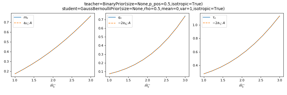
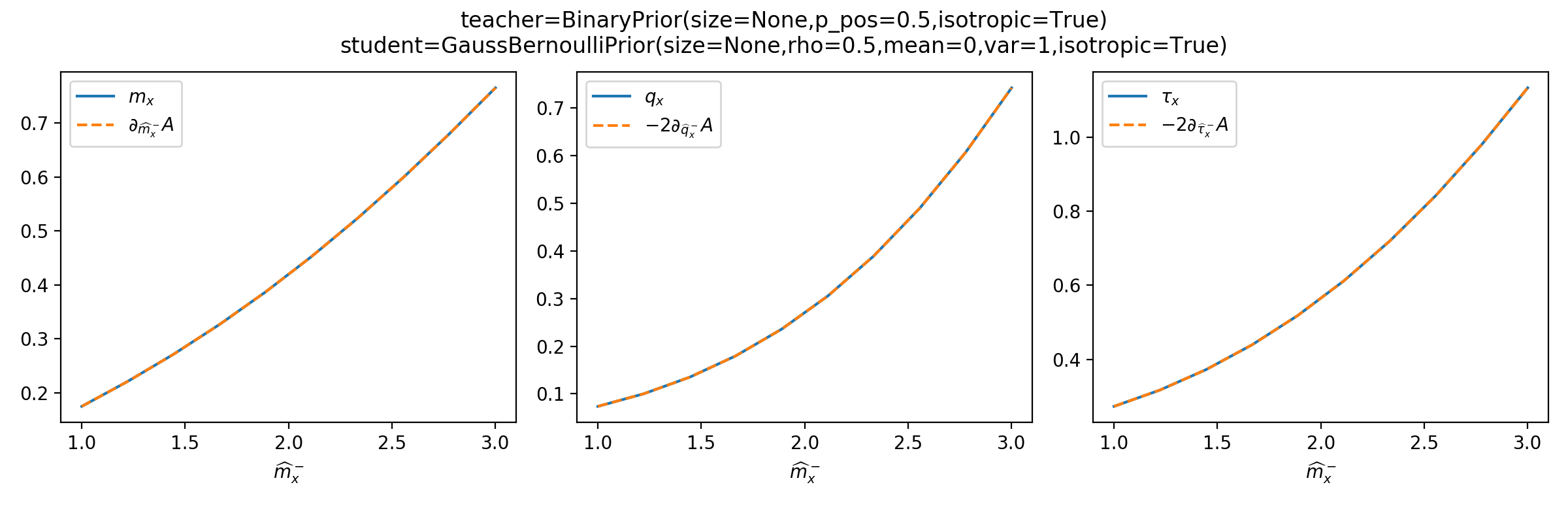
\[\begin{split}&m_x[\hat{m}_x^-,\hat{q}_x^-,\hat{\tau}_x^-] = \partial_{\hat{m}_x^-} A_p[\hat{m}_x^-,\hat{q}_x^-,\hat{\tau}_x^-] , \\ &q_x[\hat{m}_x^-,\hat{q}_x^-,\hat{\tau}_x^-] = -2\partial_{\hat{q}_x^-} A_p[\hat{m}_x^-,\hat{q}_x^-,\hat{\tau}_x^-] , \\ &\tau_x[\hat{m}_x^-,\hat{q}_x^-,\hat{\tau}_x^-] = -2\partial_{\hat{\tau}_x^-} A_p[\hat{m}_x^-,\hat{q}_x^-,\hat{\tau}_x^-] .\end{split}\]

As a sanity check, you can use tramp.checks.plot_prior_grad_EP() to check the gradients \(m_x = \partial_{\hat{m}_x^-} A_p\), \(q_x = -2\partial_{\hat{q}_x^-} A_p\) and \(\tau_x = -2 \partial_{\hat{\tau}_x^-} A_p\).

>>> from tramp.checks import plot_prior_grad_RS
>>> from tramp.priors import BinaryPrior
>>> teacher = BinaryPrior(size=None)
>>> student = GaussBernoulliPrior(size=None)
>>> plot_prior_grad_RS(teacher, student)

(png, hires.png, pdf)

Bayes-optimal¶

In the Bayes-optimal setting, the teacher generative model (a factor graph) exactly matches the student one, in particular the teacher and student priors are identical \(p(x) = p^{(0)}(x)\). In that case, we have several simplications:

\[\tau_x = \tau_x^{(0)} , \quad \hat{\tau}_x^- = \hat{\tau}_x^{-(0)} , \quad m_x = q_x = \tau_x^{(0)} - v_x , \quad \hat{m}_x^- = \hat{q}_x^- = a_x^- - \hat{\tau}_x^{-(0)}.\]

The ensemble average log-partition (free entropy) and variance \(v_x\) are then given by:

\[A_p[\hat{m}_x^-] = \mathbb{E}_{ p^{(0)}(x, b_x^-) } \, A_p[a_x^-,b_x^-] , \quad v_x[\hat{m}_x^-] = \mathbb{E}_{ p^{(0)}(x, b_x^-) } \, v_x[a_x^-,b_x^-] ,\]

and are already implemented in the base Prior class as the methods:

prior.compute_potential_BO() for \(A_p[\hat{m}_x^-]\),
prior.compute_forward_v_BO() for \(v_x[\hat{m}_x^-]\).

However you still need to implement the ensemble average over \(p^{(0)}(x, b_x^-)\), provided by the method prior.b_measure(), as in the replica symmetric mismatched case.

During state evolution, the prior receives the natural parameter message \(\lambda_x^- = \hat{m}_x^-\) and returns the moments \(\mu_x = m_x\). Actually in Tree-AMP we parametrize the message using \(a_x^- = \hat{m}_x^- + \hat{\tau}_x^{-(0)}\) instead of \(\hat{m}_x^-\) and we return the variance \(v_x\) instead of the overlap \(m_x = \tau_x^{(0)} - v_x\).

The overlap \(m_x\) is conjugate to \(\hat{m}_x^-\):

\[m_x[\hat{m}_x^-] = 2 \partial_{\hat{m}_x^-} A_p\hat{m}_x^-]\]

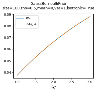
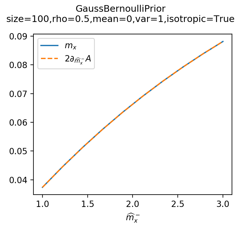
As a sanity check, you can use tramp.checks.plot_prior_grad_EP() to check the gradient \(m_x = 2 \partial_{\hat{m}_x^-} A_p\).

>>> from tramp.checks import plot_prior_grad_BO
>>> plot_prior_grad_BO(prior)

(png, hires.png, pdf)

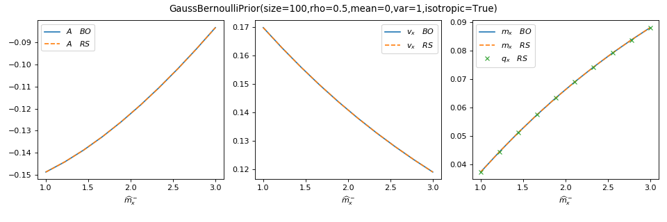
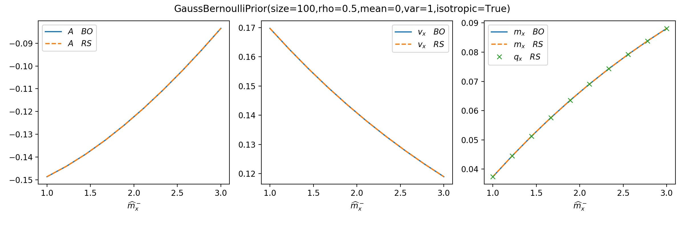
You can use tramp.checks.plot_prior_BO_limit() to check the Bayes-optimal (BO) limit of the replica symmetric (RS) potential.

>>> from tramp.checks import plot_prior_BO_limit
>>> plot_prior_BO_limit(prior)

(png, hires.png, pdf)

Bayes-optimal + Bayesian network¶

In that setting, the teacher generative model is identical to the student one, and is furthermore a Bayesian network instead of a generic factor graph. Besides the simplications occuring in the Bayes-optimal setting, we further have \(\hat{\tau}_x^{-(0)} = 0\) as the generative model is a Bayesian network, therefore:

\[m_x = q_x = \tau_x^{(0)} - v_x , \quad \hat{m}_x^- = \hat{q}_x^- = a_x^-.\]

The ensemble average log-partition (free entropy) \(A_p\), variance \(v_x\), overlap \(m_x\) and mutual information \(I_p\) are then given by:

\[\begin{split}&A_p[a_x^-] = \mathbb{E}_{ p(x, b_x^-) } \, A_p[a_x^-,b_x^-] , \\ &v_x[a_x^-] = \mathbb{E}_{ p(x, b_x^-) } \, v_x[a_x^-,b_x^-] , \\ &m_x[a_x^-] = \tau_x^{(0)} - v_x[a_x^-] , \\ &I_p[a_x^-] = \frac{1}{2} a_x^- \tau_x^{(0)} - A_p[a_x^-] .\end{split}\]

with \(p(x, b_x^-) = p(x) \mathcal{N}(b_x^- | a_x^- x, a_x^-)\) and are already implemented in the base Prior class as the methods:

prior.compute_free_energy() for \(A_p[a_x^-]\),
prior.compute_forward_error() for \(v_x[a_x^-]\),
prior.compute_mutual_information() for \(I_p[a_x^-]\),
prior.compute_forward_overlap() for \(m_x[a_x^-]\).

However you still need to implement the ensemble average over \(p(x, b_x^-)\), provided by the method:

prior.beliefs_measure() which returns \(\mathbb{E}_{p(x, b_x^-)} f(b_x^-)\) for any function \(f(b_x^-)\).

The overlap \(m_x\) (resp. variance \(v_x\)) is conjugate to the precision \(a_x^-\) for the free entropy potential \(A_p\) (resp. mutual information \(I_p\)):

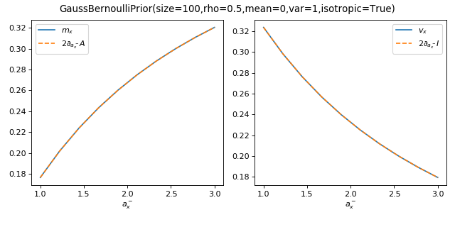
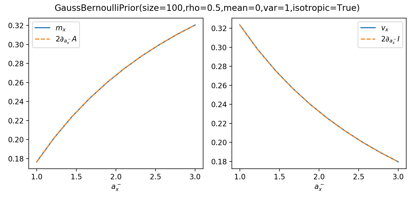
\[m_x[a_x^-] = 2 \partial_{a_x^-} A_p[a_x^-], \quad v_x[a_x^-] = 2 \partial_{a_x^-} I_p[a_x^-].\]

As a sanity check, you can use tramp.checks.plot_prior_grad_BO_BN() to check the gradients \(m_x = 2 \partial_{a_x^-} A_p\) and \(v_x = 2 \partial_{a_x^-} I_p\)

>>> from tramp.checks import plot_prior_grad_BO_BN
>>> plot_prior_grad_BO_BN(prior)

(png, hires.png, pdf)

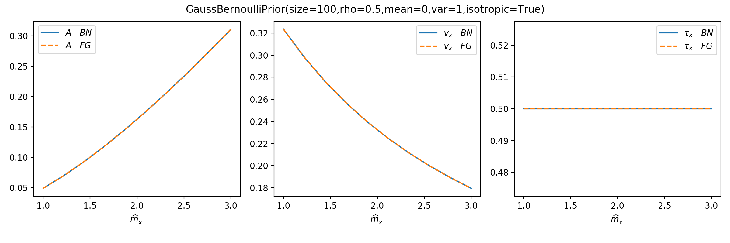
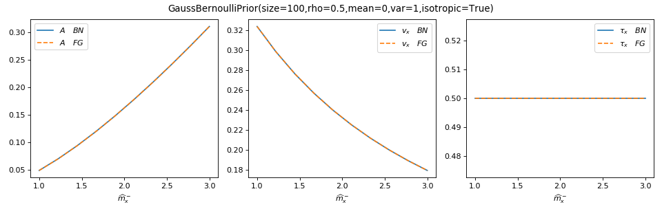
You can use tramp.checks.plot_prior_BN_limit() to check the Bayesian network (BN) limit of the Bayes-optimal but generic factor graph (FG) potential.

>>> from tramp.checks import plot_prior_BN_limit
>>> plot_prior_BN_limit(prior)

(png, hires.png, pdf)

Tests¶

If you implement a new prior for SE, please add it to the test suite tramp.tests.test_priors to make sure that it passes the gradient checking test_prior_grad_RS(), test_prior_grad_BO() and test_prior_grad_BO_BN() as well as the Bayes-optimal limit test_prior_BO_limit() and Bayesian network limit test_prior_BN_limit().

MAP priors¶

Proximal operator¶

For any factor \(f(x) = e^{-E(x)}\) associated to a regularization penalty / energy function \(E(x)\), one can use the Laplace method to obtain the MAP approximation to the log-partition, mean and variance:

\[\begin{split}A_f[a_x^-,b_x^-] &= - \min_x E(x|a_x^-,b_x^-), \\ r_x[a_x^-,b_x^-] &= x^* = \mathrm{argmin}_x E(x|a_x^-,b_x^-), \\ v_x[a_x^-,b_x^-] &= \mathrm{diag} E''(x^*|a_x^-,b_x^-)^{-1} ,\end{split}\]

for \(E(x|a_x^-,b_x^-) = E(x)+\frac{1}{2} x \cdot a_x^- x - b_x^- \cdot x\) and where \(E''(x|a_x^-,b_x^-)\) denotes the Hessian. These quantities can be expressed as:

\[\begin{split}A_f[a_x^-,b_x^-] &= \frac{\Vert b_x^-\Vert^2}{2a_x^-} - \mathcal{M}_{\tfrac{1}{a_x^-}E}\left( \frac{b_x^-}{a_x^-} \right), \\ r_x[a_x^-,b_x^-] &= \mathrm{prox}_{\tfrac{1}{a_x^-}E}\left( \frac{b_x^-}{a_x^-} \right), \\ v_x[a_x^-,b_x^-] &= \frac{1}{a_x^- } \nabla \mathrm{prox}_{\tfrac{1}{a_x^-}E}\left( \frac{b_x^-}{a_x^-} \right)\end{split}\]

where we introduce the Moreau envelop \(\mathcal{M}_g(y) = \min_x \{g(x) + \tfrac{1}{2}\Vert x-y \Vert^2\}\) and the proximal operator \(\mathrm{prox}_g(y)=\mathrm{argmin}_x \{g(x)+\tfrac{1}{2}\Vert x-y \Vert^2\}\).

Also the mean \(r_x\), variance \(v_x\) and self-overlap \(q_x=r_x^2\) are given by the gradients:

\[r_x[a_x^-,b_x^-] = \partial_{b_x^-} A_f[a_x^-,b_x^-], \quad v_x[a_x^-,b_x^-] = \partial^2_{b_x^-} A_f[a_x^-,b_x^-], \quad q_x[a_x^-,b_x^-] = -2 \partial_{a_x^-} A_f[a_x^-,b_x^-].\]

Note

For a regular prior \(p\) we have \(\tau_x = r_x^2 + v_x = -2\partial_{a_x^-} A_p\) while for a MAP prior \(f\) we have \(q_x = r_x^2 = -2\partial_{a_x^-} A_f\)

Vectorized versions¶

The vectorized versions are implemented in Tree-AMP as the methods:

prior.compute_log_partition() for \(A_f[a_x^-,b_x^-]\),
prior.compute_forward_posterior() for \(r_x[a_x^-,b_x^-]\) and \(v_x[a_x^-,b_x^-]\).

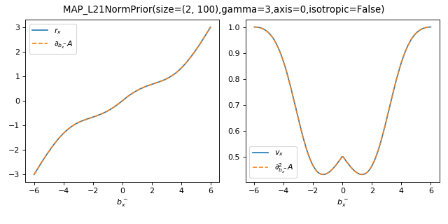
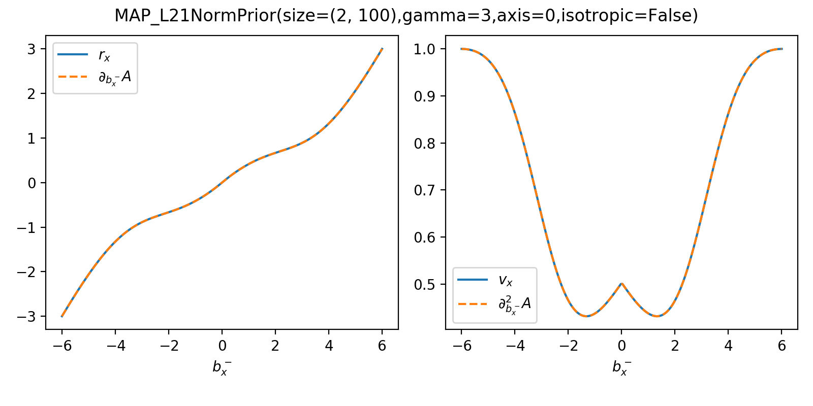
As a sanity check, you can use tramp.checks.plot_prior_grad_EP_diagonal() to check the gradients \(r_x = \partial_{b_x^-} A_f\) and \(v_x = \partial^2_{b_x^-} A_f\) for the vectorized versions, as illustrated here for the MAP_L21NormPrior associated to the \(\Vert . \Vert_{2,1}\) penalty.

>>> from tramp.checks import plot_prior_grad_EP_diagonal
>>> from tramp.priors import MAP_L21NormPrior
>>> L21_prior = MAP_L21NormPrior(size=(2, 100), gamma=3, isotropic=False)
>>> plot_prior_grad_EP_diagonal(L21_prior)

(png, hires.png, pdf)

Scalar versions¶

If the penalty is separable \(E(x) = \sum_{i=1}^{N_x} E(x^{[i]})\), for example the \(\Vert . \Vert_1\) penalty is separable but not the \(\Vert . \Vert_{2,1}\) penalty, you can define the scalar versions:

\[\begin{split}A_f[a_x^-,b_x^-] &= - \min_x E(x|a_x^-,b_x^-) = - E(x^*|a_x^-,b_x^-), \\ r_x[a_x^-,b_x^-] &= \mathrm{argmin}_x E(x|a_x^-,b_x^-) = x^* = \mathrm{prox}_{\tfrac{1}{a_x^-}E}\left( \frac{b_x^-}{a_x^-} \right) , \\ v_x[a_x^-,b_x^-] &= \frac{1}{a_x^- } \mathrm{prox}^\prime_{\tfrac{1}{a_x^-}E}\left( \frac{b_x^-}{a_x^-} \right) ,\end{split}\]

for the scalar function \(E(x|a_x^-,b_x^-) = E(x)+\frac{1}{2} a_x^- x^2 - b_x^- x\) and scalar proximal operator. They are implemented in Tree-AMP as the methods:

prior.scalar_log_partition() for \(A_p[a_x^-,b_x^-]\),
prior.scalar_forward_mean() for \(r_x[a_x^-,b_x^-]\),
prior.scalar_forward_variance() for \(v_x[a_x^-,b_x^-]\).

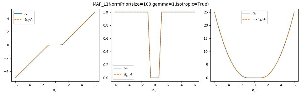
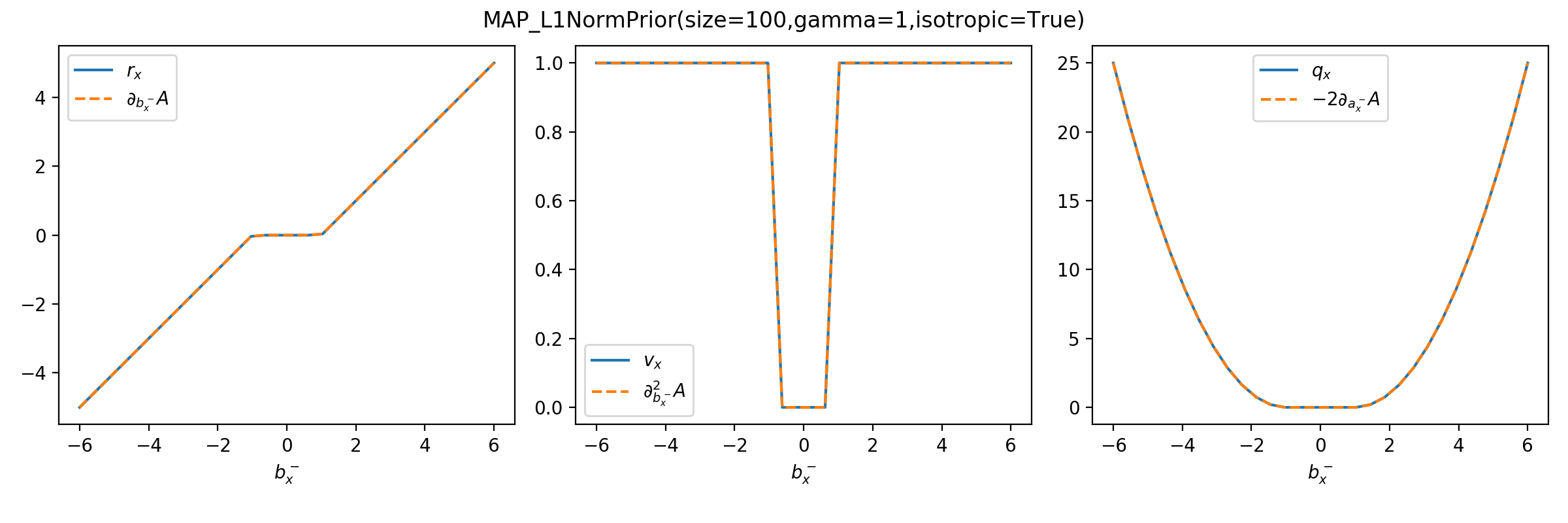
As a sanity check, you can use tramp.checks.plot_prior_grad_EP_scalar() to check the gradients \(r_x = \partial_{b_x^-} A_f\), \(v_x = \partial^2_{b_x^-} A_f\) and \(q_x = r_x^2 = -2 \partial_{a_x^-} A_f\), as illustrated here for the MAP_L1NormPrior associated to the \(\Vert . \Vert_1\) penalty.

>>> from tramp.checks import plot_prior_grad_EP_scalar
>>> from tramp.priors import MAP_L1NormPrior
>>> L1_prior = MAP_L1NormPrior(size=100)
>>> plot_prior_grad_EP_scalar(L1_prior)

(png, hires.png, pdf)

Tests¶

If you implement a new MAP prior for EP, please add it to the test suite tramp.tests.test_priors to make sure that it passes the gradient checking test_prior_grad_EP_scalar() for a separable penalty or test_prior_grad_EP_diagonal() for a non separable one.

Committee priors¶

Todo

Committee priors, covariance / precision matrix between experts