Tutorial¶

This simple guide can help you start working with Tree-AMP.

Building your first model¶

Creating a variable¶

Let us start by creating our first variable tramp.variables.SISOVariable V of size N drawn from a priors.GaussBernoulliPrior separable prior with sparsity rho

>>> from tramp.variables import SISOVariable as V
>>> from tramp.priors import GaussBernoulliPrior
>>> N, rho = 100, 0.1
>>> prior = GaussBernoulliPrior(size=N, rho=rho)
>>> var_x = prior @ V("x")

The opeartor @ allows to assign a variable x drawn from a prior distribution, and in general to concatenate modules together.

Draw a matrix from an ensemble¶

Creating a matrix W instance of the tramp.ensembles.GaussianEnsemble of size M x N can be done by

>>> from tramp.ensembles import GaussianEnsemble
>>> M, N = 200, 100
>>> ensemble = GaussianEnsemble(M, N)
>>> W = ensemble.generate()

Constructing a linear channel¶

The variable x can be mutliplied by the matrix W using the channels.LinearChannel. The result can be casted in a new variable z0 = W x with W ~ ensemble and x ~ prior.

>>> from tramp.channels import LinearChannel
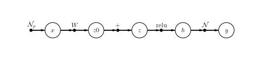
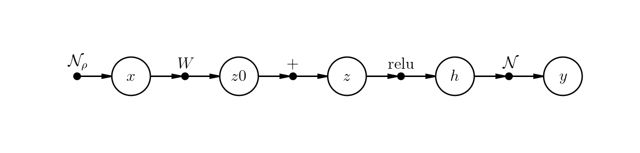
>>> model = prior @ V("x") @ LinearChannel(W=W, name='W') @ V("z0")

Adding other modules¶

As many module as desired can be added to the previous model. Each module must be followed by a variable V. For example a tramp.channels.BiasChannel with value b with intermediate variabel z, followed by a tramp.channels.ReluChannel outputing a variable h.

>>> from tramp.channels import BiasChannel, ReluChannel
>>> b = 0.1
>>> model = model @ BiasChannel(bias=b) @ V("z")
>>> model = model @ ReluChannel() @ V("h")

Adding observations¶

Observations tramp.SILeafVariable O can be added to the the model. For example model may go through a noisy tramp.channels.GaussianChannel with variance var and outputs a variable y

>>> from tramp.variables import SILeafVariable as O
>>> from tramp.channels import GaussianChannel
>>> var = 1e-2
>>> model = model @ GaussianChannel(var=var) @ O("y")

Representing the model¶

Once the model completed, it can be built with the method .to_model() and drawn with .plot() :

>>> model = model.to_model()
>>> model.plot()

(png, hires.png, pdf)

EP/SE in the Bayes-optimal scenario¶

Let us illustrate how to run EP or SE in the Bayes-optimal case and on a more complex model: a sparse gradient prior.

Build the model¶

Creating a variable x of size N sampled from a tramp.priors.GaussianPrior with n_next=2 successors can be done with a tramp.variables.SIMOVariable V

>>> from tramp.variables import SIMOVariable as V
>>> from tramp.priors import GaussianPrior
>>> N = 100
>>> prior_x = GaussianPrior(size=N, var=1) @ V(id="x", n_next=2)

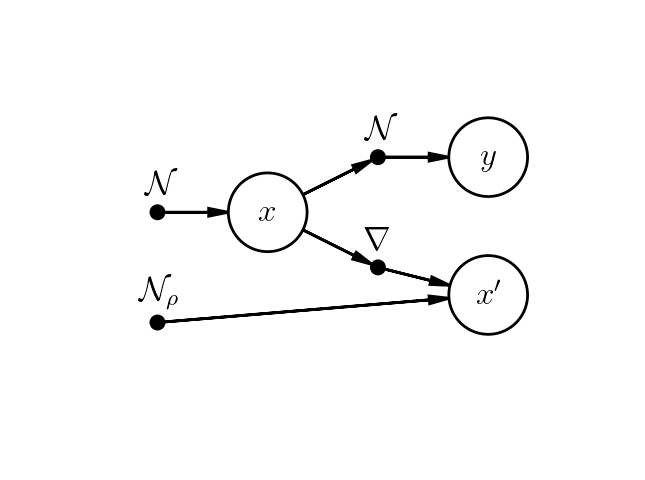
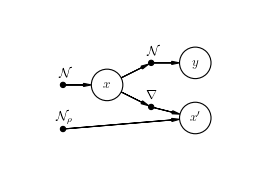
which can be connected to a tramp.channels.GaussianChannel with y observations and a sparse gradient constraint on x. This constraint can be built with a new variable x' connected to n_prev=2 predecesors: a tramp.channels.GradientChannel connected to x and a tramp.priors.GaussBernoulliPrior with sparsity rho.

>>> from tramp.channels import GradientChannel, GaussianChannel
>>> from tramp.priors import GaussBernoulliPrior
>>> from tramp.variables import SISOVariable as V, MILeafVariable
>>> rho = 0.04
>>> var = 0.1
>>> x_shape = (N,)
>>> grad_shape = (1,) + x_shape
>>> # Create the gaussian channel and the observations y
>>> channel_y = GaussianChannel(var=var) @ O("y")
>>> # Create the sparse gradient constraint and the new variable x'
>>> channel_grad = (GradientChannel(shape=x_shape) + GaussBernoulliPrior(size=grad_shape, rho=rho)) @ MILeafVariable(id="x'", n_prev=2)
>>> # Plug the two channels to the variables x
>>> model = prior_x @ ( channel_y +  channel_grad )
>>> # Build the model
>>> model = model.to_model()
>>> # Show the model
>>> model.plot()

(png, hires.png, pdf)

Teacher-Student scenario¶

In a tramp.experiments.BayesOptimalScenario, ground truth samples of all the variables contained in the model are drawn (namely x, x', y ). The scenario tries then to infer the variables x_ids from the observations y and knowing the structure and the parameters of the model (rho, var). The scenario is setup with a .setup() method where an optional seed can be used for reproducibility.

>>> from tramp.experiments import BayesOptimalScenario
>>> x_ids = ["x", "x'"]
>>> scenario = BayesOptimalScenario(model, x_ids=x_ids)
>>> scenario.setup(seed=42)

Run Expectation Propagation (EP)¶

EP can be run on the above scenario with the method .run_ep(). Optional maximum number of iterations max_iter and damping on all variables to help convergence can be added. Different callback can be used such as tramp.algos.EarlyStoppingEP if precision tol is reached.

>>> from tramp.algos import EarlyStoppingEP
>>> scenario.run_ep(max_iter=1000, damping= 0.1, callback=EarlyStoppingEP(tol=1e-2))

To use multiple callbacks at a time, you need to use tramp.algos.JoinCallback:

>>> from tramp.algos import JoinCallback, EarlyStoppingEP, TrackOverlaps, TrackEstimate
>>> track_overlap = TrackOverlaps(true_values=scenario.x_true)
>>> track_estimate = TrackEstimate()
>>> callback = JoinCallback([track_overlap, track_estimate, EarlyStoppingEP(tol=1e-12)])

Run State Evolution (SE)¶

SE can be performed simply with the run_se() method

>>> scenario.run_se()

Todo

Continue the tutorial