Beliefs

A belief is specified by the base space \(X\) as well as the chosen set of sufficient statistics \(\phi(x)\). Any variable type defines an exponential family distribution

\[p(x|\lambda) = e^{\lambda^\intercal \phi(x) - A(\lambda)}\]

indexed by the natural parameter \(\lambda\). We will denote by \(b \in \lambda\) the natural parameter associated to the statistic \(x \in \phi(x)\). The log-partition, mean and variance are then given by:

\[A(\lambda) = \ln \int_X dx e^{\lambda^\intercal \phi(x)}, \quad r(\lambda) = \partial_b A(\lambda), \quad v(\lambda) = \partial_b^2 A(\lambda)\]

The second moment is given by \(\tau(\lambda) = r(\lambda)^2 + v(\lambda)\)

In Tree-AMP, a belief is implemented as a python submodule of tramp.beliefs containing the functions A(), r(), v(), tau() and some additional functions if relevant. As a sanity check, you can use the tramp.checks.plot_belief_grad_b() that will check that \(r = \partial_b A\) and \(v = \partial_b^2 A\). See the various beliefs below for concrete examples.

If you implement a new belief, please make sure that it passes the gradient checking and add it to the test suite tramp.tests.test_beliefs.test_belief_grad_b().

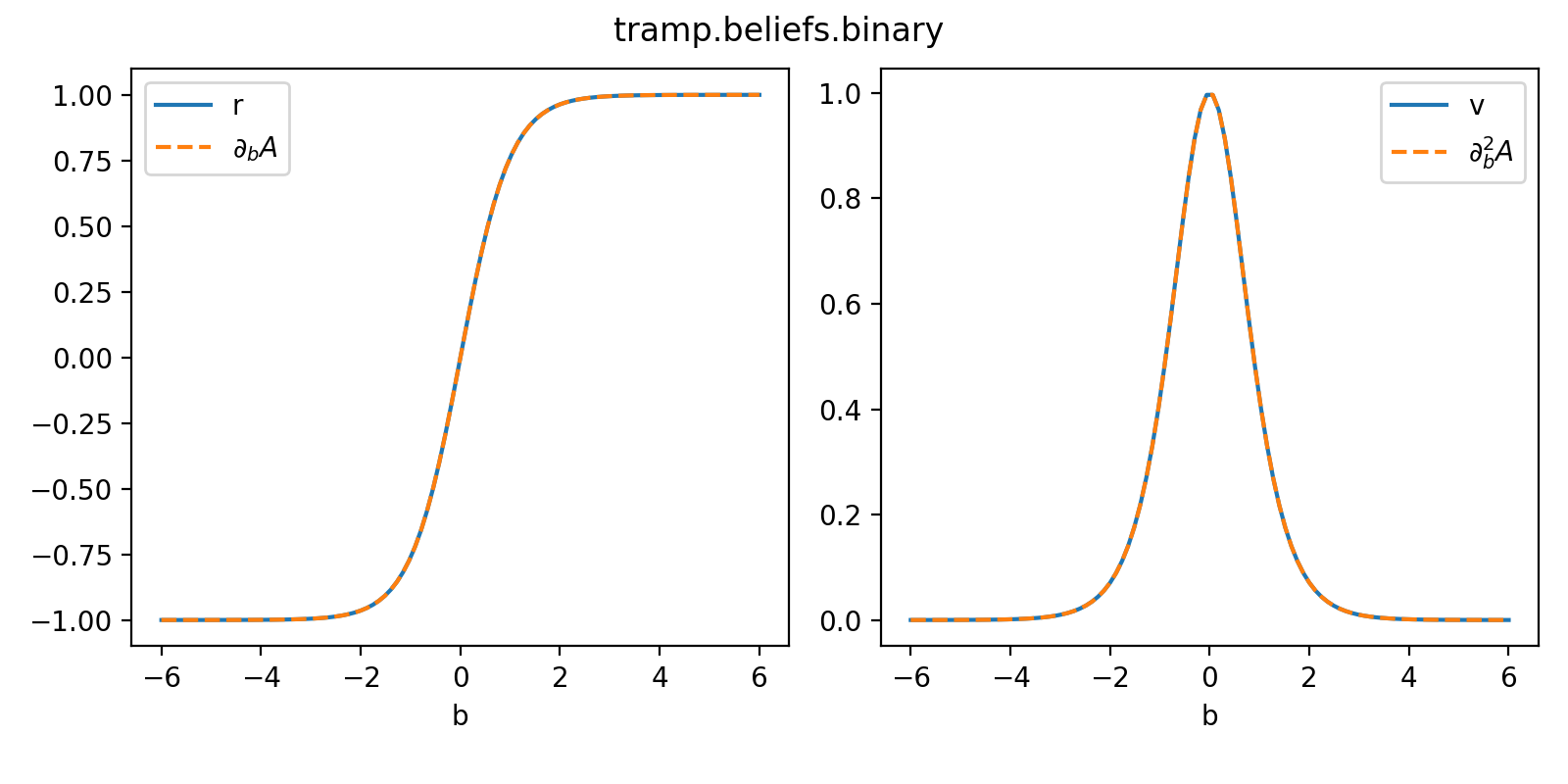
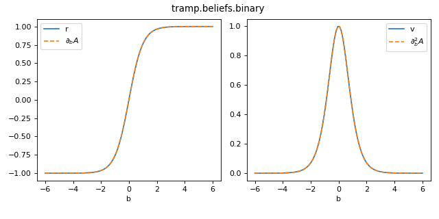
Binary

The log-partition, mean and variance are given by

\[A(b) = \ln (e^{+b} + e^{-b}), \quad r(b) = \tanh(b), \quad v(b) = 1-\tanh(b)^2\]

The corresponding exponential family distribution is the Bernoulli

\[p(x|b) = p_+ \delta_+(x) + p_- \delta_-(x)\]

where the natural parameter \(b = \tfrac{1}{2}\ln\tfrac{p_+}{p_-}\) is (half) the log-odds.

>>> from tramp.beliefs import binary
>>> from tramp.checks import plot_belief_grad_b
>>> plot_belief_grad_b(binary)

(png, hires.png, pdf)

tramp.beliefs.binary.A(b)

tramp.beliefs.binary.r(b)

tramp.beliefs.binary.v(b)

tramp.beliefs.binary.tau(b)

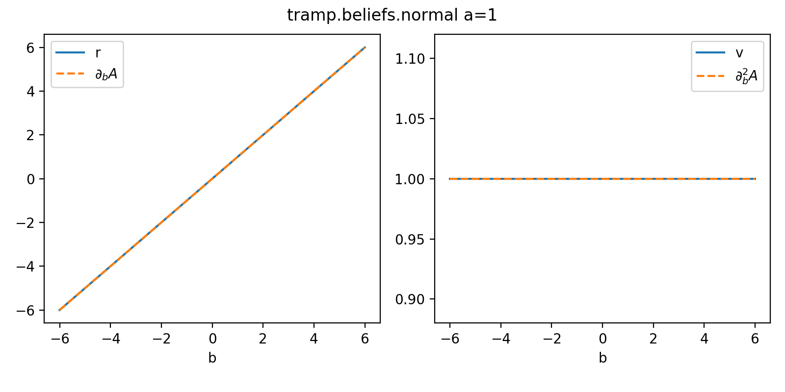
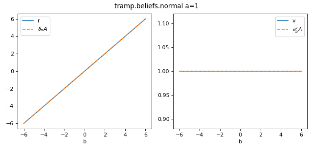
Normal

The log-partition, mean and variance are given by

\[A(a,b) = \frac{b^2}{2a} + \frac{1}{2} \ln \frac{2\pi}{a}, \quad r(a,b) = \frac{b}{a}, \quad v(a,b) = \frac{1}{a}\]

The corresponding exponential family distribution is the Normal

\[p(x|a,b) = \mathcal{N}(x|r,v)\]

of mean \(r=\frac{b}{a}\) and variance \(v=\frac{1}{a}\)

>>> from tramp.beliefs import normal
>>> from tramp.checks import plot_belief_grad_b
>>> plot_belief_grad_b(normal, a=1)

(png, hires.png, pdf)

tramp.beliefs.normal.A(a, b)

tramp.beliefs.normal.r(a, b)

tramp.beliefs.normal.v(a, b)

tramp.beliefs.normal.tau(a, b)

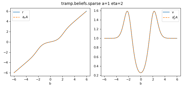
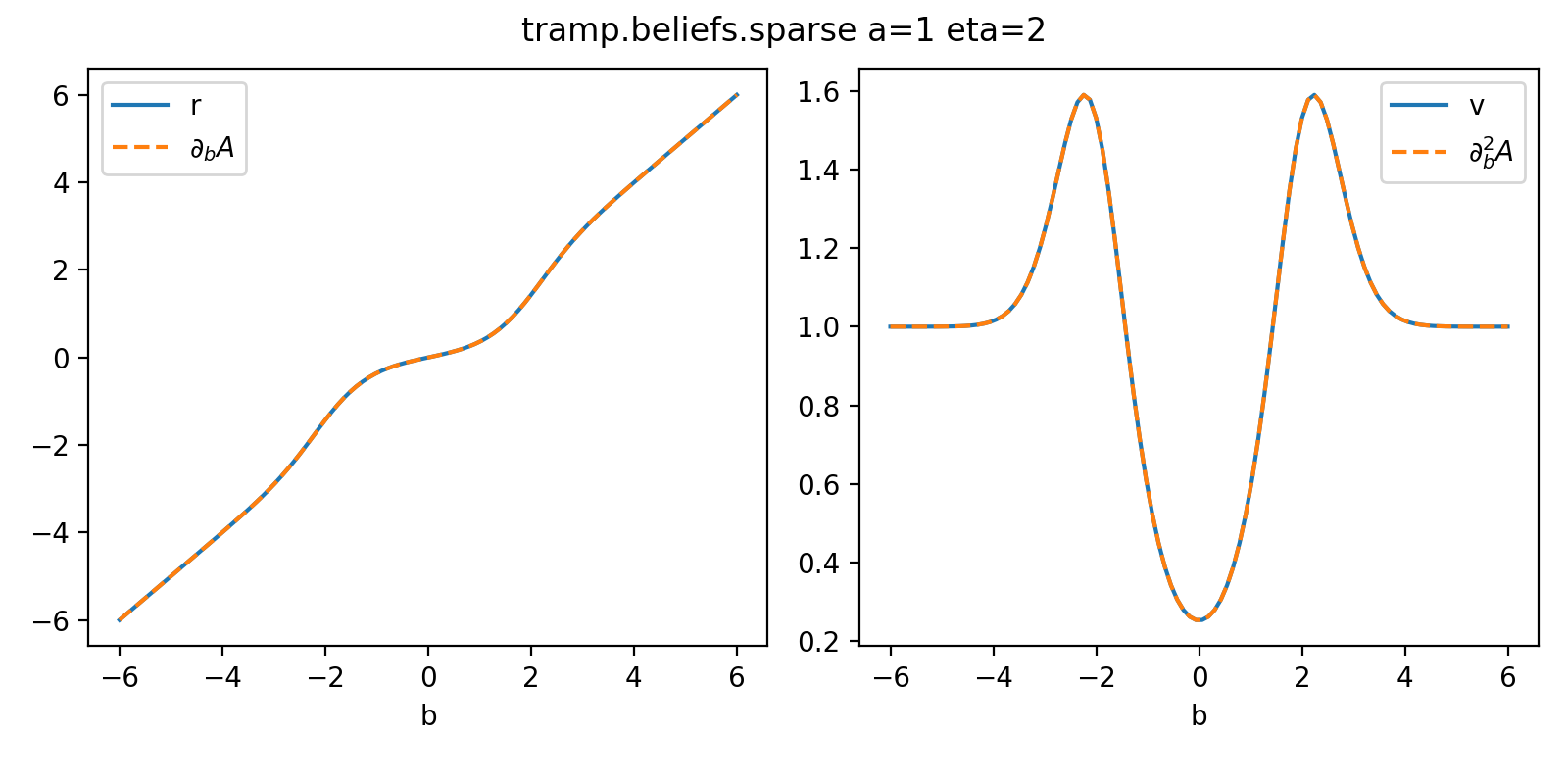
Sparse

The log-partition, mean and variance are given by

\[A(a,b,\eta) = \ln (e^{\eta} + e^{A(a,b)}), \quad r(a,b,\eta) = \sigma(\xi)r, \quad v(a,b,\eta) = \sigma(\xi)v + \sigma(\xi)(1-\sigma(\xi))r^2\]

where \(A(a,b), r=r(a,b), v=v(a,b)\) are the log-partition, mean and variance of a Normal variable, \(\sigma(\xi)\) is the sigmoid and \(\xi = A(a,b) - \eta\).

Besides there is a finite probability \(p(x=0 | a,b,\eta) = 1 - \sigma(\xi)\) that \(x\) is exactly zero. We will denote its complementary by

\[p(a,b,\eta) = p(x \neq 0 | a,b,\eta) = \sigma(\xi)\]

The corresponding exponential family distribution is the Gauss-Bernoulli

\[p(x|a,b,\eta) = [1 - \rho] \delta_0(x) + \rho \mathcal{N}(x|r,v)\]

with fraction of non-zero elements \(\rho = p(a,b,\eta)\)

>>> from tramp.beliefs import sparse
>>> from tramp.checks import plot_belief_grad_b
>>> plot_belief_grad_b(sparse, a=1, eta=2)

(png, hires.png, pdf)

tramp.beliefs.sparse.A(a, b, eta)

tramp.beliefs.sparse.r(a, b, eta)

tramp.beliefs.sparse.v(a, b, eta)

tramp.beliefs.sparse.tau(a, b, eta)

tramp.beliefs.sparse.p(a, b, eta)

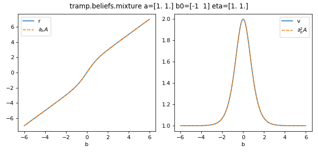
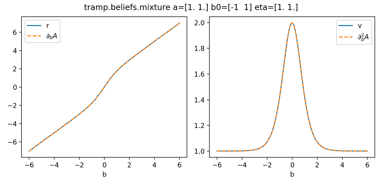
Mixture

We consider a K-mixture Normal variable with natural parameters \(a = \{a_k\}_{k=1}^K\), \(b = \{b_k\}_{k=1}^K\) and \(\eta = \{\eta_k\}_{k=1}^K\). The log-partition, mean and variance are given by

\[A(a,b,\eta) = \ln \sum_k e^{\xi_k}, \quad r(a,b,\eta) = \sum_k \sigma_k r_k, \quad v(a,b,\eta) = \sum_k \sigma_k v_k + \sum_{k<l} \sigma_k \sigma_l [r_k - r_l]^2\]

where \(A(a_k, b_k), r_k = r(a_k, b_k), v_k = v(a_k, b_k)\) are the log-parition, mean and variance of the \(k^{th}\) Normal variable, \(\sigma = \mathrm{softmax}(\xi)\) and \(\xi_k = \eta_k + A(a_k, b_k)\).

Besides the probability to belong to each of the K-components is

\[p_k(a,b,\eta) = p(x \in k | a,b,\eta) = \sigma_k\]

The corresponding exponential family distribution is the Gaussian mixture

\[p(x|a,b,\eta) = \sum_k \sigma_k \mathcal{N}(x|r_k,v_k)\]

On the plot below, the gradients of \(A(a,b+b_0,\eta)\) are taken with respect to scalar \(b\) for fixed 2-components \(a, b_0, \eta\) and are checked against the corresponding \(r(a,b+b_0,\eta)\) and \(v(a,b+b_0,\eta)\).

>>> from tramp.beliefs import mixture
>>> from tramp.checks import plot_belief_grad_b
>>> plot_belief_grad_b(mixture, a=np.ones(2), b0=np.array([-1, +1]), eta=np.ones(2))

(png, hires.png, pdf)

tramp.beliefs.mixture.A(a, b, eta)

tramp.beliefs.mixture.r(a, b, eta)

tramp.beliefs.mixture.v(a, b, eta)

tramp.beliefs.mixture.tau(a, b, eta)

tramp.beliefs.mixture.p(a, b, eta)

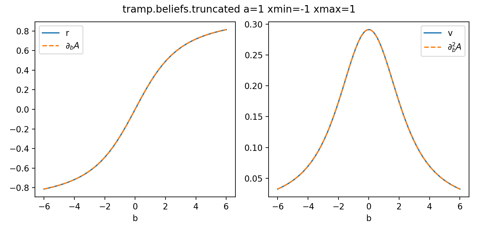
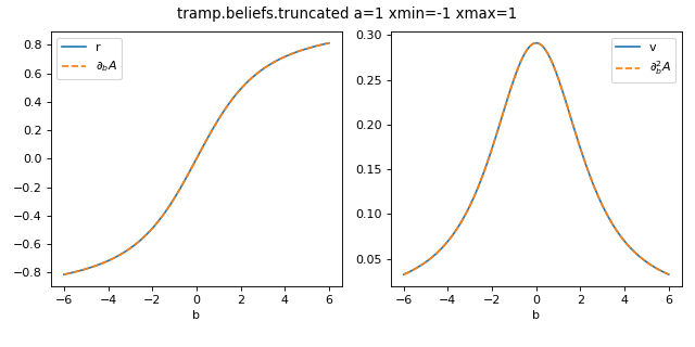
Truncated

We consider a truncated Normal variable restricted to the interval \(X = [x_\min, x_\max]\). The log-partition, mean and variance are given by

\[A_X(a,b) = A(a,b) + \ln p_Z, \quad r_X(a,b) = r + \sqrt{v} r_Z , \quad v_X(a,b) = v v_Z\]

where \(A(a,b), r=r(a,b), v=v(a,b)\) are the log-partition, mean and variance of a Normal variable.

\(p_Z\) denotes the probabilty that the standard Normal \(z \sim \mathcal{N}(0,1)\) falls withing the rescaled interval \(Z = \frac{X - r}{\sqrt{v}} = [z_\min, z_\max]\)

\[p_Z = \int_Z dz \mathcal{N}(z) = \Phi(z_\max) - \Phi(z_\min)\]

with \(\Phi\) the Normal cumulative distribution function.

It is equal to the probabilty \(p_X(r, v)\) that the Normal \(x \sim \mathcal{N}(r, v)\) falls within the \(X\) interval:

\[p_X(r, v)= \int_X dx \mathcal{N}(x | r, v) = p_Z\]

\(r_Z\) denotes the mean and \(v_Z\) the variance of the standard Normal \(z \sim \mathcal{N}(0,1)\) restricted to the \(Z\) interval:

\[r_Z = \frac{\mathcal{N}(z_\min)-\mathcal{N}(z_\max)}{\Phi(z_\max)-\Phi(z_\min)} , \quad v_Z = 1 - r_Z^2 + \frac{z_\min \mathcal{N}(z_\min)-z_\max \mathcal{N}(z_\max)}{\Phi(z_\max)-\Phi(z_\min)}\]

Warning

Computing \(r_Z\), \(v_Z\) and \(\ln p_Z\) is numerically tricky, especially in the tails. We follow the implementation suggested in the TruncatedNormal.jl Julia package.

The corresponding exponential family distribution is the truncated Normal

\[p(x|a,b) = \mathcal{N}_X(x|r,v) = \frac{1}{p_X(r, v)} 1_X(x) \mathcal{N}(x|r,v)\]

>>> from tramp.beliefs import truncated
>>> from tramp.checks import plot_belief_grad_b
>>> plot_belief_grad_b(truncated, a=1, xmin=-1, xmax=1)

(png, hires.png, pdf)

tramp.beliefs.truncated.A(a, b, xmin, xmax)

tramp.beliefs.truncated.r(a, b, xmin, xmax)

tramp.beliefs.truncated.v(a, b, xmin, xmax)

tramp.beliefs.truncated.tau(a, b, xmin, xmax)

tramp.beliefs.truncated.p(a, b, xmin, xmax)

Probabilty that x ~ N(r, v) with r=b/a and v=1/a falls within [xmin, xmax]

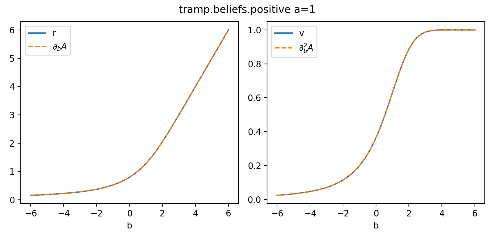
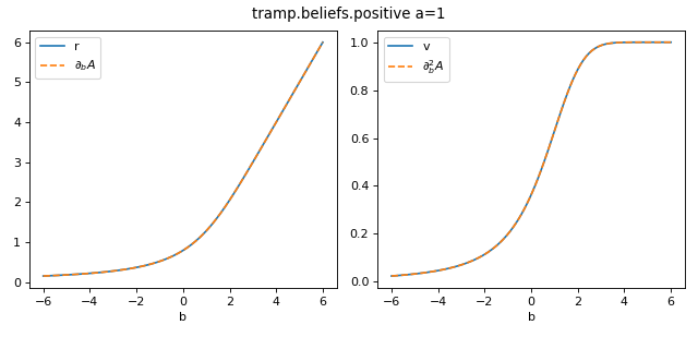
Positive

It corresponds to a Normal variable resticted to \(X=\mathbb{R}_+\) and a special case of the Truncated variable with \(x_\min=0\) and \(x_\max = +\infty\).

>>> from tramp.beliefs import positive
>>> from tramp.checks import plot_belief_grad_b
>>> plot_belief_grad_b(positive, a=1)

(png, hires.png, pdf)

tramp.beliefs.positive.A(a, b)

tramp.beliefs.positive.r(a, b)

tramp.beliefs.positive.v(a, b)

tramp.beliefs.positive.tau(a, b)

tramp.beliefs.positive.p(a, b)

Probabilty that x ~ N(r, v) with r=b/a and v=1/a falls within R_+

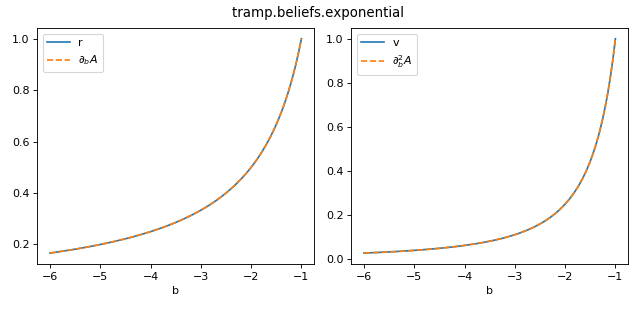
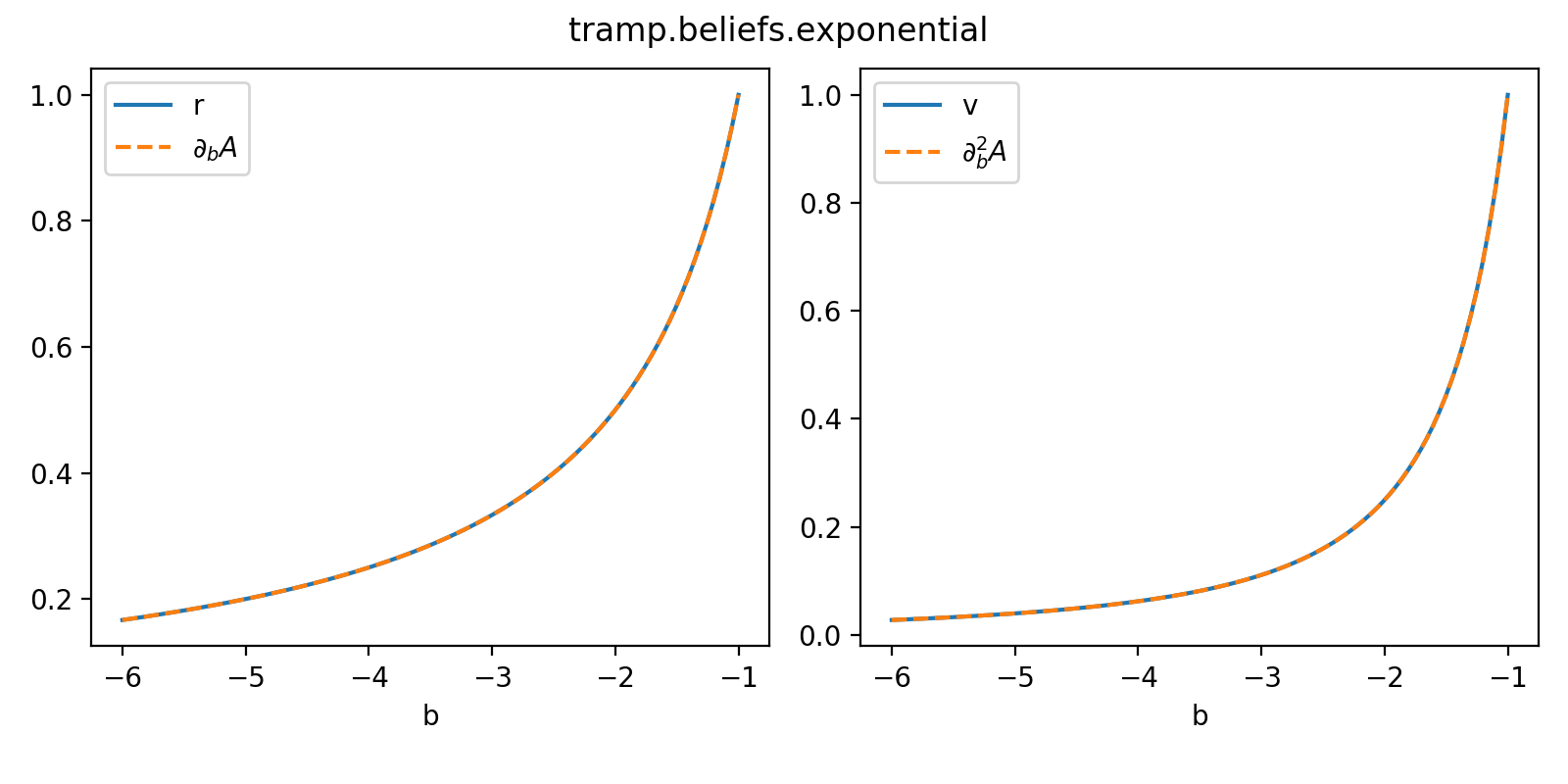
Exponential

The log-partition, mean and variance are given by

\[A(b) = - \ln (-b) , \quad r(b) = -\frac{1}{b} , \quad v(b) = \frac{1}{b^2}\]

The corresponding exponential family distribution is the Exponential with mean \(r = -\frac{1}{b}\)

\[p(x|b) = 1_{\mathbb{R}_+}(x) \frac{1}{r} e^{- \frac{x}{r} }\]

The Exponential variable is also the limit \(a\rightarrow 0\) of the Positive variable:

\[p(x|b) = \lim_{a\rightarrow 0} p_{\mathbb{R}_+}(x | a,b)\]

Note

The natural parameter \(b\) must be negative.

>>> from tramp.beliefs import exponential
>>> from tramp.checks import plot_belief_grad_b
>>> plot_belief_grad_b(exponential)

(png, hires.png, pdf)

tramp.beliefs.exponential.A(b)

tramp.beliefs.exponential.r(b)

tramp.beliefs.exponential.v(b)

tramp.beliefs.exponential.tau(b)