Perceptron

import pandas as pd
from tramp.algos import EarlyStoppingEP
from tramp.models import glm_generative
from tramp.experiments import BayesOptimalScenario, qplot, plot_compare

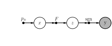
Model

We wish to infer the binary signal \(x \sim \mathrm{Bin}( . | p_+) \in \pm^N\) from \(y = \mathrm{sgn}(Fx) \in \pm^M\), where \(F \in \mathbb{R}^{M \times N}\) is a Gaussian random matrix. You can build the perceptron directly, or use the glm_generative model builder.

teacher = glm_generative(
    N=1000, alpha=1.7, ensemble_type="gaussian", prior_type="binary",
    output_type="sgn"
)
scenario = BayesOptimalScenario(teacher, x_ids=["x"])
scenario.setup(seed=42)
scenario.student.plot()

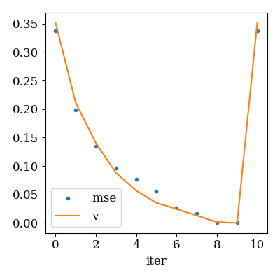
EP dynamics

ep_evo = scenario.ep_convergence(
    metrics=["mse"], max_iter=30, callback=EarlyStoppingEP()
)
qplot(
    ep_evo, x="iter", y=["mse", "v"],
    y_markers=[".", "-"], y_legend=True
)

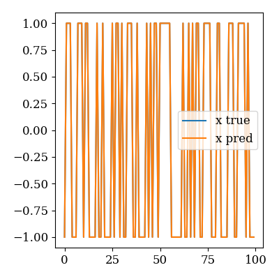
Recovered signal

plot_compare(scenario.x_true["x"], scenario.x_pred["x"])

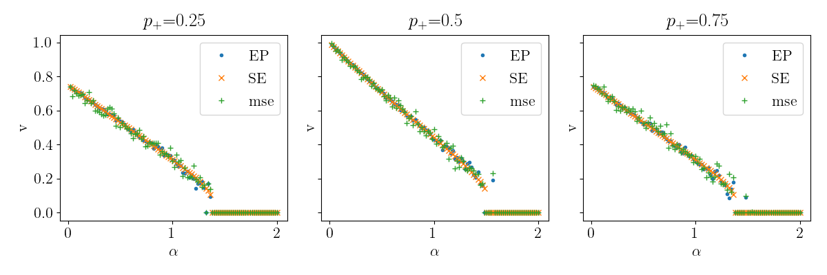
Compare EP vs SE

See data/perceptron_ep_vs_se.py for the corresponding script.

rename = {
    "alpha": r"$\alpha$", "n_iter": "iterations", "p_pos": r"$p_+$", "source=": ""
}
df = pd.read_csv("data/perceptron_ep_vs_se.csv")
qplot(
    df, x="alpha", y="v", marker="source", column="p_pos",
    rename=rename, usetex=True, font_size=16
)

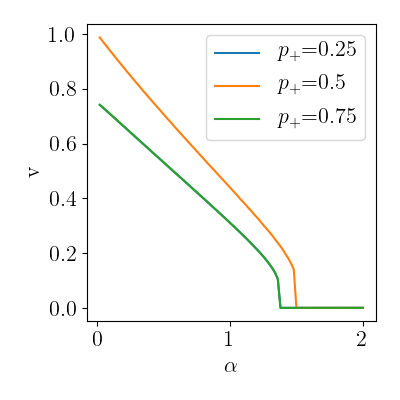
Phase transition

qplot(
    df.query("source=='SE'"), x="alpha", y="v", color="p_pos",
    rename=rename, usetex=True, font_size=16
)

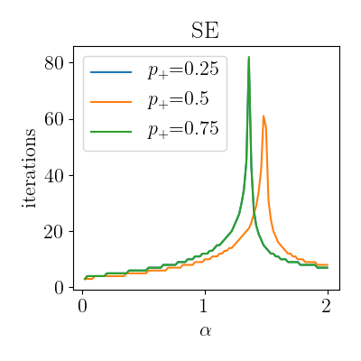
Number of iterations diverging at the critical value

qplot(
    df.query("source=='SE'"),
    x="alpha", y="n_iter", color="p_pos", column="source",
    rename=rename, usetex=True, font_size=16
)